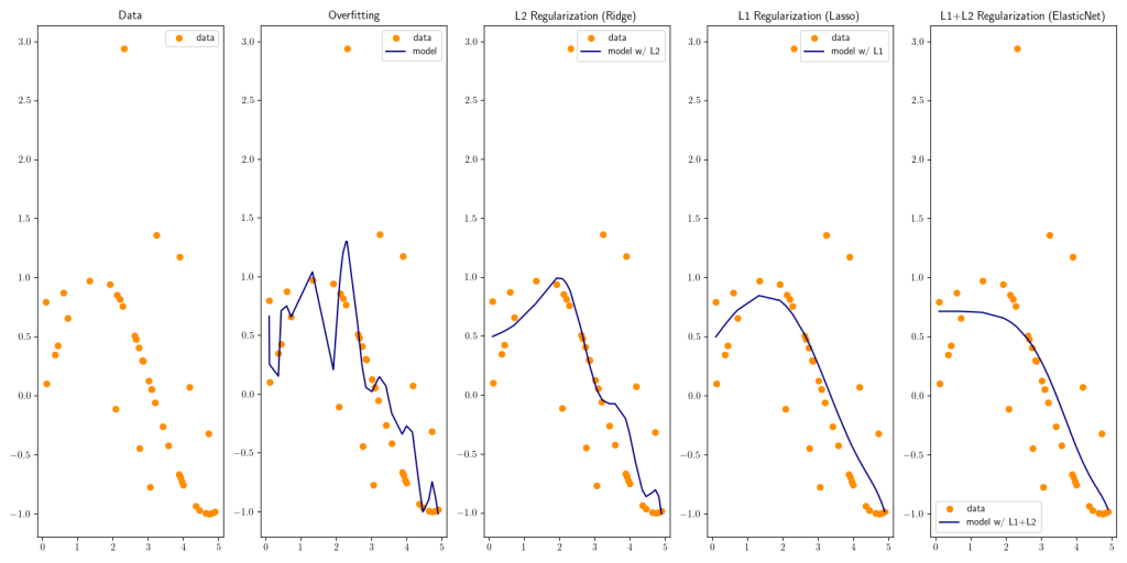
In order to mitigate overfitting our linear model we can add one or more regularization terms to our loss function. The regularization terms incentivize lower the weights in the coefficient/weight matrices.
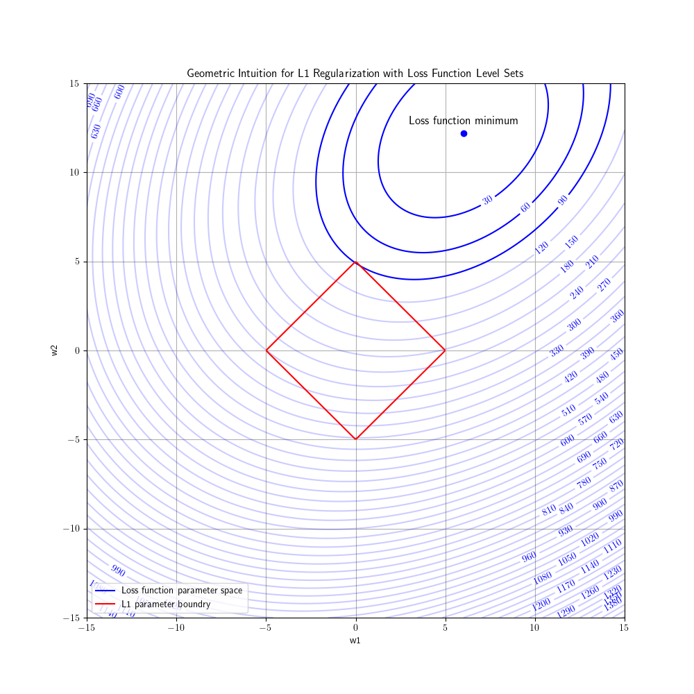
Why does one want to avoid large coefficients? When you have large weights in you model this lead to high variance. Imagine having the equation:
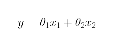
If we try setting the θ1 to different values, we can see how it will affect y:

As we can see when the weights is large, small perturbations in the input data x will yield massive effect on the y, the model has high variance. These perturbations can be noise captured from real-world sensors and we don’t want the noise to dominate our predictions. Also it makes interpretability harder, because we don’t know if the model puts large emphasis on certain features due to noise or because it is really important.
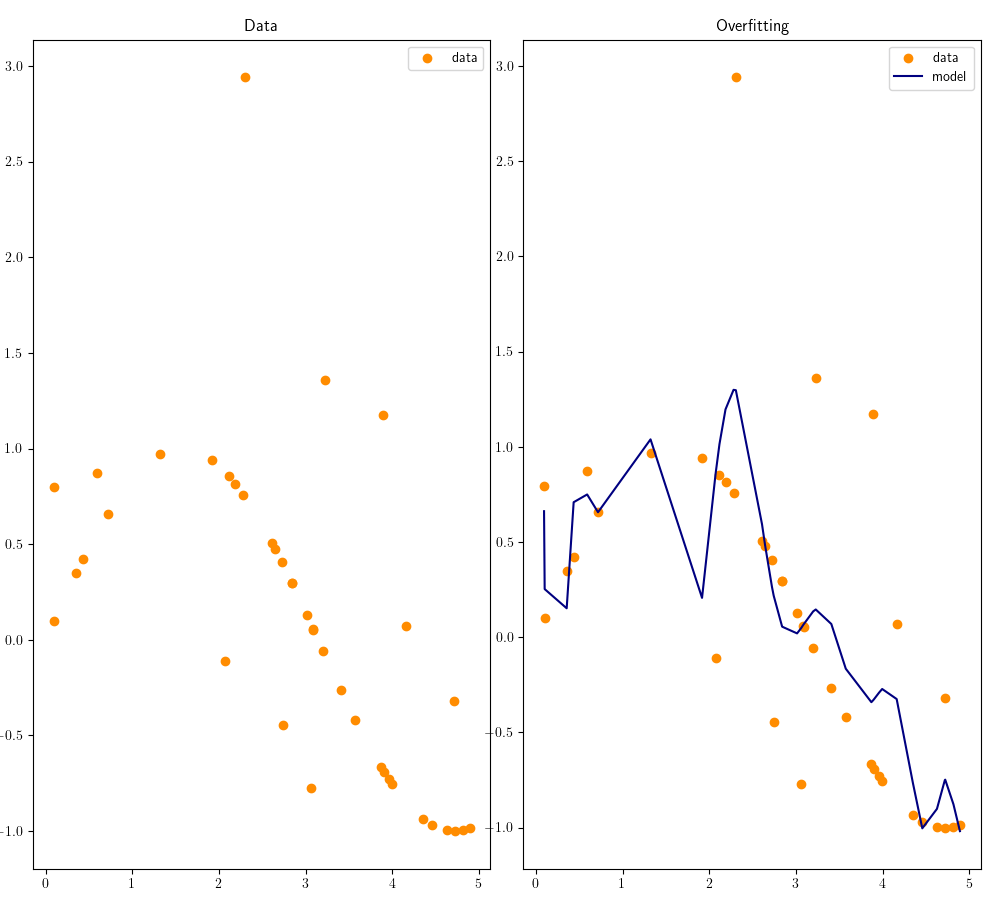
Here is an other example one can see how the outliers affect the model, instead of the model being a smooth curve it gets edgy by treating the data points with lots of noise as regular data points. The model is overfitting the data by incorporating all the noise, which leads to an unstable model with large coefficients:
One way to mitigate overfitting is to penalize large weights during training. This can be done in multiple ways, but one of them is to add one or more regularization terms, R, to our loss function, L:
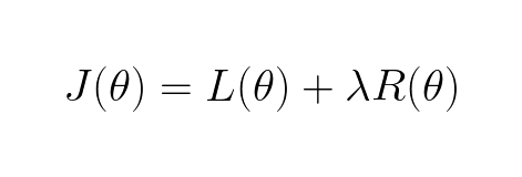
The lambda is a hyperparameter (meaning its defined by the user) which scales the regularization term. The three most common regularization terms are:
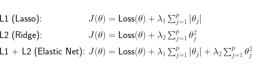
L1 (Lasso) regularization adds the sum of absolute values of each of coefficient/weight to the loss. Large values whether negative or positive increases the loss substantially, so during training it avoids searching parameter spaces where the parameters/weights/coefficients are big. One characteristic of the L1 regularization is that often makes some of the weights to zero. To understand why this happens we can take a look at the geometrical representation of the L1 regularization:
In the figure above we se that the optimal weights are where a loss function parameter level set intersect with the L1 parameter boundry. As we can see below in the figure, which depict a model with two weights, the intersection is when w1 = 0 and w2 = 5. This is a great reduction of weights given the global minimum for the loss function are when w1 = 6 and w2 = 12.
L2 (Lasso) regularization adds the sum of the coefficients squared to the loss. One characteristic of the L2 loss is that it heavily penalize large weights, if a weight is 10 it will add 100 to the loss compared to L1 which would only add 10 to the loss. This heavy penalization of large weight can easily be seen if we visualize the parameter space of the loss function with the L2 regularization in 3D:
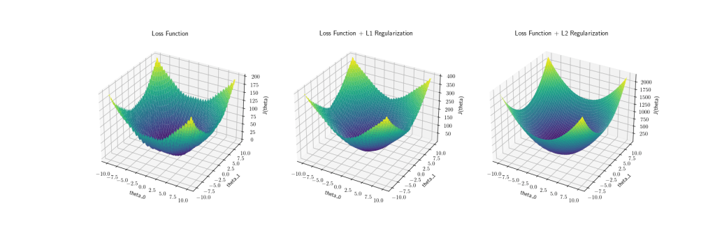
In the figure above we can see in the L2 loss the higher the weights the penalize much heavier (2000) than L1 loss (400). Another characteristic of L2 loss is that the weights tend to be non-zero. This can be seen more easily when looking at the geometrical representation of the L2 loss:
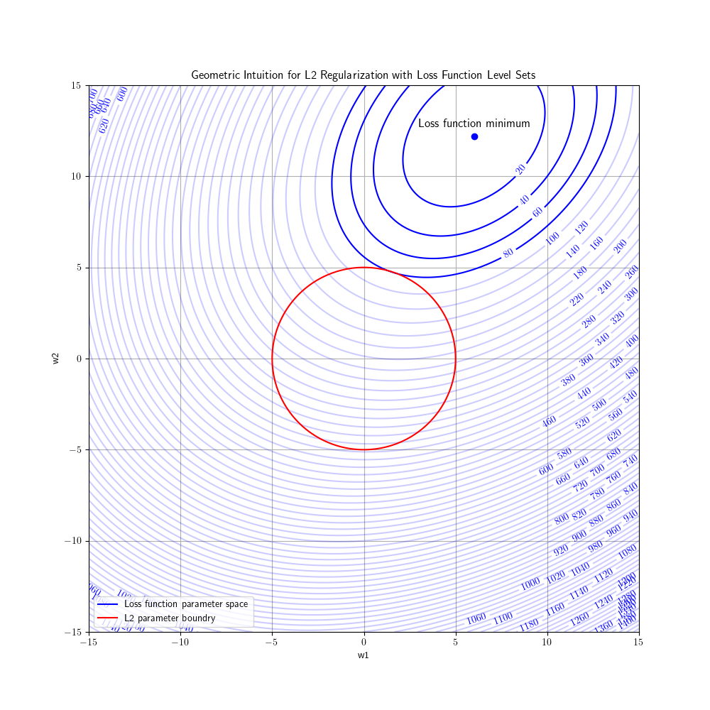
In the figure above we see that in the optimal solution for L2 loss w1 become small but not zero, w2 becomes a little less than 5.
Lastly, we have the L1+L2 loss which is just the combination of L1 and L2 loss.
To summarize we can look at the effect L1, L2 and L1+L2 have on the model when utilized: