kbclock.work

Sometimes it useful to predict a class given input data, unlike in linear and polynomial regression where you predict a number given input data. To predict binary class labels (either 1 or 0) one can use logistic regression.

Its worth noting that while polynomial regression is kind of a extension of linear regression, logistic regression does not have as strong connection to linear regression, yet there are some similarities; e.g. both use a linear combination of features as decision function and they can use same numerical optimizers (gradient descent, newton, etc) to find the optimal weights.

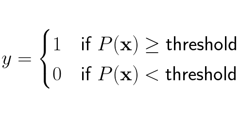
The path to find logistic regression is a great example of mathematical modelling, it comprises many different math concepts but is not too extensive. Let’s start modelling! Firstly, in logistic regression one wants the output to be one of two classes/labels, lets say we deal with class 1 and class 0. In logistic regression we want to estimate the probability for the class 1 given input features x, we call the estimated probability P. Since P is a probability it ranges from 0 to 1, and whenever P is over a given threshold (usually 0.5) the data point x is classified as 1.

Formally we can write the estimated probability for x as:

Lets focus on the probability for getting the label 1 given input vector x:

Given this probability for getting label 1 we can determine its class, so we want to create a model that outputs this value. One way to model this probability is to assume we can model this probability as a linear combination of each element in the input vector x:

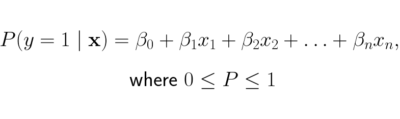
The issue with this model is that we strongly restrict what the linear expression can be when it only can be between 0 and 1. This reduces the solution space of the linear expression, only some linear combinations will be in the range 0 to 1. To increase the solution space we can make the left side be the odds (the ratio between the probability of an event happening and it not happening) of y = 1 instead of the probability of y = 1:

This will expand the output range of the linear expression from [0,1] to [0, ∞]. This is better but the solution space of the linear expression is still limited to whole numbers. To make sure the linear expression can be any rational number [-∞, ∞], thus increasing its solution space further, we take the natural logarithm of the odds:

Now the linear expression on the right hand side don’t need to impose any restrictions, whatever the linear expression yields is acceptable! This expression should let us be able to capture to the linear relationship between the estimated class probability and the features in a data point. To get an expression as for the probability we rewrite the expression into:

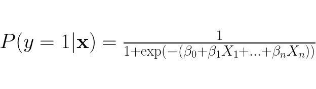
The right hand side is the sigmoid function, which always yields a value between 0 and 1. Fun fact, the usage of the sigmoid function in machine learning stems from logistic regression.

Now that we have an expression for the estimated probability for y = 1, we need a measure that tells us how well our estimated probabilities are with respect to the actual labels y = 1. When the label is 1 for a data point we want the the estimated probability that y = 1 to be as high as possible, thus we want to maximize the product of the estimated probabilities that y = 1 when the label is 1. We say we maximize the likelihood function over all data points:

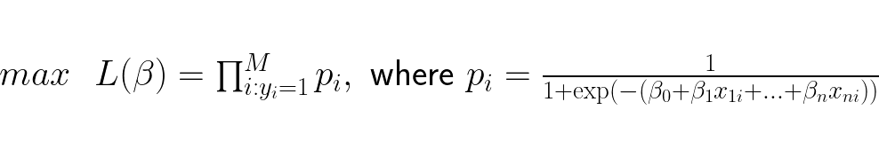
This method considers only the the data points with label 1, find their probabilities and multiply them together. The higher this number is, the better the model estimates the probability for the data point having label 1.

However, there’s a major flaw in this model design, the probability distribution is not optimized for when Y = 0. We have a lot of data points that are unused in the optimization which causes information loss. We need to optimize the probabilities for when y = 0 as well, if not the model suffers from information loss.

To utilize both label classes during optimization we need an expression that captures the estimated probabilities for both y = 1 and y = 0. Luckily type of dataset we have, where the output is discrete (no decimal numbers) and there are only two possible outcomes (1 or 0), have the Bernoulli distribution. It can be represented mathematically by the Probability Mass Function (PMF):

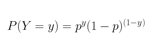
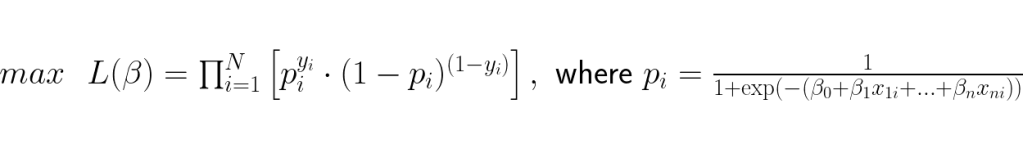
This expression has everything we need; it takes into account the estimated probability for each of our label values. When the label is 1 it will yield the probability that x has Y = 1 and when the label is 0 it will yield the probability that x has Y = 0. Using this expression we can optimize the weights by maxing its likelihood function, which in the case where all data point labels is covered is called Maximum Likelihood Estimation (MLE):

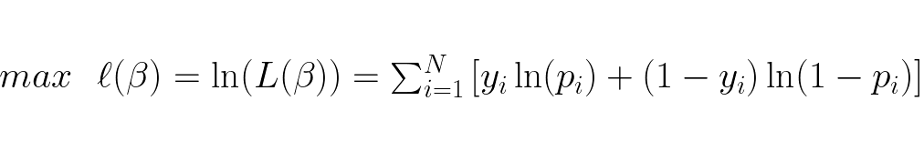
Maximizing the function finds the optimal weights, however the function is not computationally optimal. The accumulated probabilities can become extremely small and computers may not be able to represent these numbers which would lead to round off errors. To counter this we take the log of the likelihood function and obtain the log-likelihood function which transforms it from being a product of terms to a sum of terms:

It can be proved that the Hessian matrix of this log-likelihood function is a negative semi-definite matrix, thus it is concave and has only one global maximum. This global maximum is found when the gradient of the log-likelihood function is 0, so we need the gradient which is:

This gradient can be written very beautifully in matrix form:

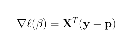
Side note, the gradient of just the likelihood (no log in front) function would not be as compact and nice in matrix form. Further, we want to find when the gradient is zero:

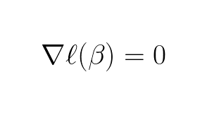
In contrast to linear and polynomial regression, the gradient of the log-likelihood function is nonlinear (because p is calculated using the sigmoid function) hence generally not possible to solve analytically. Note, some nonlinear equations can be solved analytically but these are rare and should be seen as exceptions rather then the rule. Since solving it analytically (finding the exact solution) is usually impossible, we choose a numerical approach where we approximate the solution until certain conditions is satisfied (this can be that a number of iterations is achieved, accuracy of prediction is achieved or something else).

Two fundamental numerical methods that can be used is Newton-Raphson or gradient descent. Newton-Raphson requires that the Hessian of the log-likelihood function to be invertible, this is not always the case so the safer bet would be to use gradient descent which does not have this requirement. The gradient decent expression can be written as:

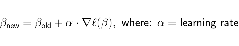
In gradient decent firstly the the weights β with random weights. Then β is updated iteratively until stop condition is met. The stop condition can be that:

• A certain number of β updates is performed.
• The increase of the log-likelihood at a update step is less than a threshold set, in other words convergence is a fact.

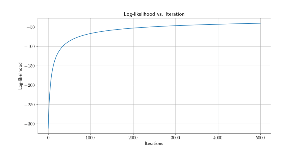
Using logistic regression we optimize weights of models so that they get higher log-likelihood with each iteration/weight update, which in turn leads to higher accuracy of the model.