kbclock.work

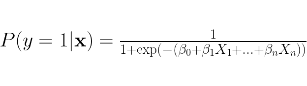
Often we want to predict the label/class of a data point where there are more than two labels. Taking a look at binary linear regression, we see it is only created for when there are only two labels to choose from. From binary logistic regression we have:

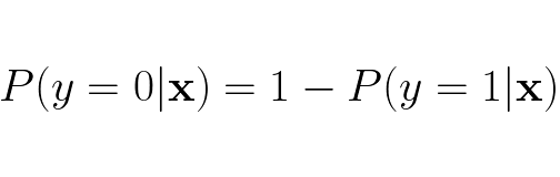
When there only two possible outcomes we can easily derive what the probability for y = 0 given feature vector x is:

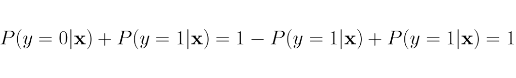
We also see that the probability nicely adds up to 1:

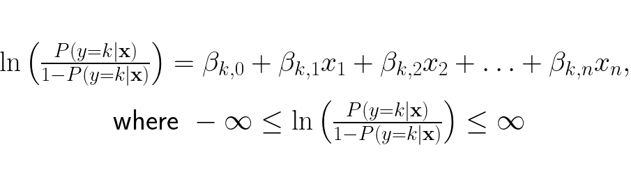
This method is explicitly made to only handle binary classification, so it is difficult to make this method to handle more classes. However, there’s hope, we can branch off from an earlier point of the modelling process of the binary logistic regression to make a version of logistic regression that can handle more than two classes. We need to revert back to this step:

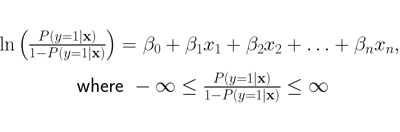
We want the odds to represent the ratio of probability for y = k and probability for y = ¬k, so we update the odds to be:

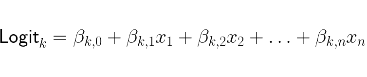
The linear expression updated is because while in binary logistic regression it is sufficient to output just one logit (logarithm of the odds of a probability) to determine the class, in multi-class regression you need one logit per class. A logit of class k is:

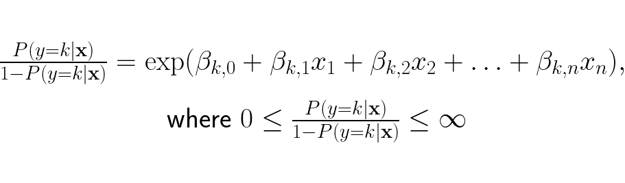
We now have the log-odds of y being any arbitrary class k. We want the odds on the right hand side not the log-loss, so we restructure the expression to be:

We can now find the odds for every k class in our dataset. Since we have an expression for the odds of each class k, we can turn the odds of each k to an expression for the probability of each k. This is achieved by dividing the odds for class k (z_k) by the sum of the odds of each class k (z_j) :

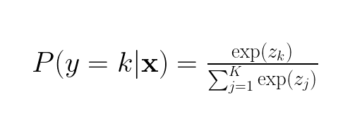
We now have function for the probability for each class, this function is called the softmax function. Now we define a likelihood function which represents the probability of observing the entire dataset given the weights β:

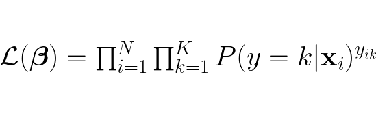
This likelihood function iterates over each datapoint x, for each x it retains the probability if the k is the same class as the label y. Each probability retained is multiplied with all the other retained probabilities, this yields the probability of observing the entire dataset given the weights β.

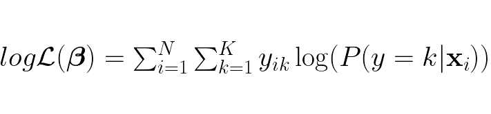
Since products are harder computationally and not as matrix friendly as sums (especially with regards to the gradient), we transform the likelihood function into the log-likelihood function:

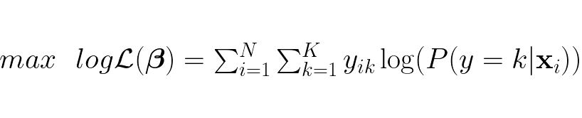
We want to maximize this function to find the optimal weights β:

To find the optimal weights we need to first find the gradient:

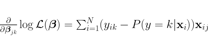
Which by the way is this in matrix format:

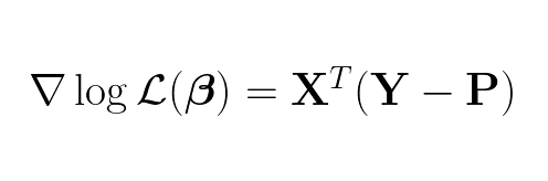
Having the gradient, we can use gradient ascent to find weights β when the gradient is 0. This β is the optimal weights for our multi-class logistic regression model.

Here is an example of a trained multi-class logistic regression model for linear separable data points:

First the data points is linearly transformed by taking the dot product of the examples and the weights, then adding the biases. The manifold is now skewed/rotated compared to the original manifold above. Then soft-max is applied which “squeezes” the data points together even more together, which results in an even more narrow/compressed manifold as seen below:

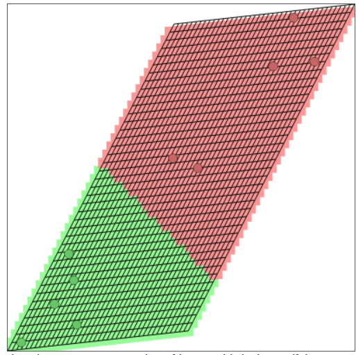
(This great tool by Andrej Karpathy is used to create visualization of the linearly transformed space/manifold.)